NeurIPS 2018 Batch Normalization

I was one of the lucky few that managed to get a NeurIPS ticket last minute off the waitlist and was excited to hear about the latest findings in ML research. Amidst the frigid Montreal weather, I saw some groundbreaking research regarding batch normalization that made a lot of researchers (and myself) re-think the reason for using batch normalization within their network architectures.

What is Batch Normalization?

For people who do not know what batch normalization is, batch normalization (BN) is a technique used with mini-batch training to normalize activation values in neural network layers by taking the output of the previous activation layer and zero-centering the batch mean and forcing unit batch variance via [1]:

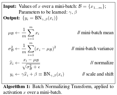
where two new trainable parameters $\gamma$ and $\beta$ are introduced that scale and shift the output via a linear transformation; we note that for an arbitrary loss $\mathcal{L}$, our backpropagation of our gradients with respect to our six new variables are continous & differentiable, thus allowing $\gamma$ and $\beta$ to be learned via an optimization method such as SGD.

The purpose of BN, as proposed in the original paper by Sergey Ioffe & Christian Szedegy [1] is the following:

When feeding outputs in one activation layer to a subsequent layer, their distributions vary during training. With varying distributions, gradient descent has a hard time finding the minima of our proposed optimization problem when each layer does not have uniform scale as gradient descent is not scale invariant. This causes our learned parameters to change from the previous layer, creating inconsistencies, and causing the need for lower learning rates to be chosen & careful weight initialization in order to create a well-conditioned environment for our model to be trained; we denote this change in the input layers’ distribution as internal covariate shift (ICS). Hence, utilizing BN reduces ICS by creating a uniform scale of our input distributions.

Ioffe & Szedegy also state that higher learning rates can be used in conjunction with BN due to the normalization of distributions across the network, causing vanishing and exploding gradients to be less likely and prevents getting stuck in local minima during training. Backpropagation gains more resilience as well, with the layer Jacobian and progagated gradients being more closer to scale invariant with respect to the weights calculated than before.

NeurIPS Findings

Even with Ioffe & & Szedegy’s explanation, there is still a lot of unknown as to what governs the behavior behind BN during training. Johan Bjorck, Carla Gomes, Bart Selman, and Kilian Q. Weinberger sought to explain experimentally BN’s behavior on training [3]. In their first experiment, they trained a 110-layer ResNet on CIFAR-10 with three different learning rates $0.0001, 0.003, 0.1$ with and without BN:

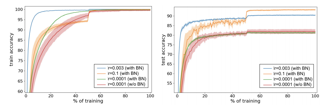
They observed that with the smallest learning rate, BN provided a small boost in training speed but both models converged to the same test accuracy, whilst the higher learning rates benefited greatly from BN, allowing for faster training without compromising test accuracy and adds regularization. Bjorck et al. attribute this to the larger learning rates generate more SGD “noise” which in turn creates a regularization effect and prevents getting stuck in sharp minima, supported by Keskar et al 2017 findings [4].

But why does using BN allow for higher learning rates? Bjorck et al. observe the relative loss during the first few mini-batches as a function of the step size:

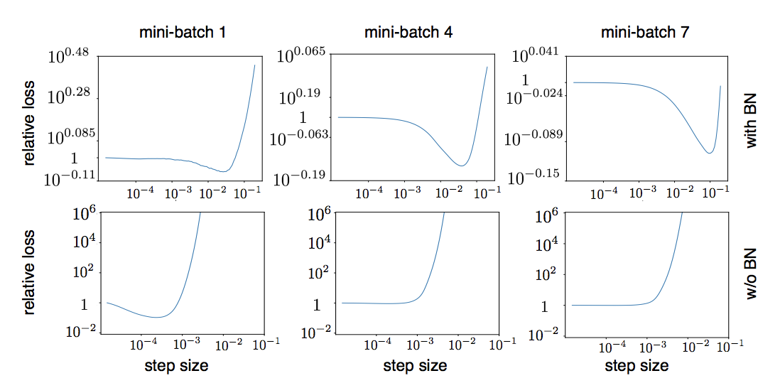
We observe that networks utilizing BN do not diverge as rapidly as networks without BN with respect to step size. Is this due to the fact that we reduce ICS or some other phenomena?

Santurkar et al. argue that their is a greater effect at play with using BN: we are smoothing our optimization landscape such that we create a further well-conditioned optimization problem that aids SGD in finding a solution. Due to creating approximately scale invariance from activation layer to activation layer, BN allows spikes and bumps in our non-convex loss function to be smoothed, thus allowing for a larger learning rate and more predictive gradients to be computed [3]. In order to measure this smoothing effect, Santurkar et al. propose the following definition:

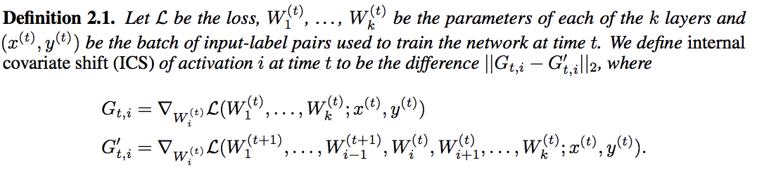
To my knowledge, this is the first proposed mathematical definition ICS, namely calculating the $l_2$ distance between the sum of all gradients of $\mathcal{L}$ with respect to our parameters $W_{k}^t$ where $G_{t,i}$ corresponds to the gradients before the layer weight update and $G_{t, i}^{'}$ responds to the gradients after the layer weight update. In their paper, they go on to prove theoretically that BN provides a more well-behaved optimization problem by inducing favorable properties such as Lipschitz continuity and increased predictive gradients [3].

Recall that for an arbitrary function $f$, we say $f$ is L-Lipschitz if $\vert f(x_1) - f(x_2) \vert \leq L \vert \vert f(x_1) - f(x_2) \vert \vert$ for all $x_1$ and $x_2$ and for some constants $L$. Intuitively, Lipschitz continuity ensures that your function does not explode at some point. We can extend this notion of reduction of explosion to the gradients of $f$ via $\beta$-smoothness where we say $f$ is $\beta$-smooth if its gradients are $\beta$-Lipschitz i.e. if $\|\nabla f(x_1)-\nabla f(x_2) \| \leq \beta \|x_1 - x_2 \|$ for some constant $\beta$.

Experimentally, Santurkar et al. used the VGG network on CIFAR-10 with & without BN, calculated the $l_2$ distance between the loss weight gradients $\vert\vert G_{t,i} - G_{t,i}^{'}\vert\vert_2$ and found the following during training:

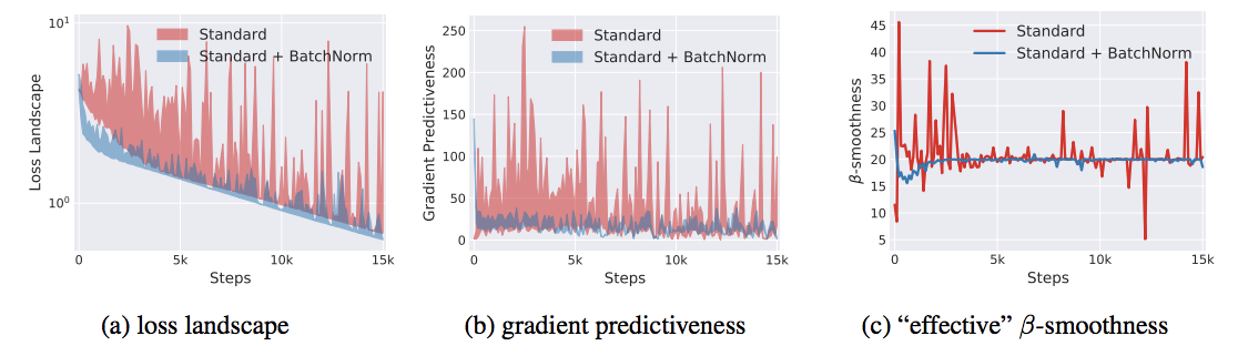
where (a) corresponds to the variation in loss function’s value, (b) is the $l_2$ disance of $G$, and (c) the maximum $l_2$ over distance moved in that direction, which we define as “effective” $\beta$-smoothness [3]. We immediately see that the addition of BN generates a smoother loss landscape by drastically reducing the fluctuations in gradient predictiveness via the created $\beta$-smoothing effect on $\mathcal{L}$.

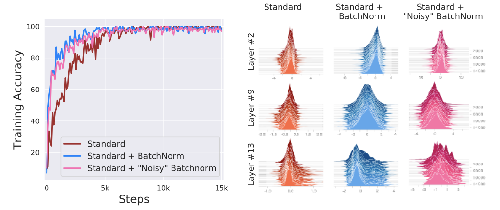
Furthermore, Santurkar et al. devised a clever experiment to examine whether ICS had anything to do with increased training performance. They trained three VGG networks on CIFAR-10: one without BN, one with BN, and one with BN where the activation, after passing the BN layer, was perturbed via i.i.d noise sampled from a time-step dependent, non-zero mean and non-unit variance distribution $D_j^{t}$ for each activation $j$ for each sample in each batch. This pertubation produces a severe covariate shift that is non-uniform across all activations that would induce a decrease in training performance. However, they observe that even though less stable distributions are produced with the noisy pertubation, training performance is not impacted:

Conclusions

We see that batch normalization’s connection to training performance and internal covariate shift is weak at best. Rather, we see that batch normalization provides another method for smoothing our optimization landscape to be more stable, thus allowing for higher learning rates to be used which in turn improves training performance. This explains the known benefits of batch normalization such as prevention of exploding / vanishing gradients and robustness to hyperparameter selection.